This project was part of a small group benchmark on foundation models for multiplexed fluorescence microscopy. The general question was simple: if we take recent pretrained models and run them on real multiplexed microscopy data, what do their embeddings actually capture?
My part focused on a channel-agnostic masked autoencoder, or CA-MAE, from the paper Masked Autoencoders for Microscopy are Scalable Learners of Cellular Biology. I did not train a new foundation model here, and I did not fine-tune the model. The work was more practical than that: take a pretrained model, make our data fit the input format, run inference on the university cluster, and then look at the resulting embeddings carefully.
That sounds straightforward in one sentence. In practice, a lot of the interesting work was in the details.
Why I Looked At This
Multiplexed fluorescence microscopy is a really rich kind of data. Instead of just one image, each cell can have many channels, where each channel corresponds to a different biological marker. That makes the data powerful, but also awkward.
Different experiments can have different marker panels. Some datasets have more channels, some have fewer, and the channels are not always in the same order or even measuring the same thing. So a normal image model with a fixed input layout is not always a great fit.
That is why the channel-agnostic idea was interesting to me. In principle, a model like CA-MAE should be more flexible about the number and order of microscopy channels. For a project like this, that sounded very useful: instead of training a custom model for every dataset, maybe we could use a pretrained model as a general feature extractor.
The big question was whether that actually worked well enough on our data.
The Model I Tried
CA-MAE is based on the masked autoencoder idea. During training, parts of the image are hidden, and the model learns to reconstruct them. The version from the paper is adapted for microscopy data, where channels matter a lot more than in ordinary RGB images.
For this project, I used the pretrained model as a frozen feature extractor. The code for my project branch is private, but the public model code and paper are from Recursion’s maes_microscopy repository.
The model can produce different kinds of representations. I mainly looked at three:
- a global embedding for the whole cell image
- channel-level embeddings, where each selected marker gets its own representation
- local patch embeddings, where smaller regions of the image are embedded separately
I liked this part because it made the project feel less like a black box. Instead of only asking “does the model work?”, I could ask what changes when I look at the cell level, the channel level, or the patch level.
What I Actually Had To Do
The first real step was not analysis. It was getting the image data into the shape the model expected.
The available inference setup had a practical constraint: I worked with 11 input channels. Our microscopy data did not naturally come as exactly those 11 channels. Some datasets had more channels, and not every channel was equally useful for the question we wanted to ask. So I had to choose a subset that made biological sense and also worked technically.
That sounds like a small preprocessing detail, but it mattered. The channel choice affected what the model could see. If the selected markers were too narrow, the embeddings would miss important structure. If the selection was too broad or inconsistent, comparisons became harder to interpret.
After that came the usual but important image handling:
- load the microscopy arrays
- select the chosen channels
- normalize each channel
- resize the images to the model input size
- run batched inference on the cluster
- save embeddings and metadata for later analysis
For the stem-cell-style data, there was also a maximum-intensity-projection step to turn focal stacks into 2D images. That was another reminder that “use a foundation model” still leaves a lot of work around the edges. The model only sees the final tensor. The choices before that point are still on you.
Looking At The Embeddings
Once the embeddings were saved, I used UMAP and Leiden clustering to inspect them. I treated these as exploratory tools, not as final proof of anything. UMAP plots can be useful, but they are also easy to overread.
The first thing I wanted to know was whether the embeddings separated the biological conditions we cared about. For the broader cell-state differences, the global embeddings looked more useful. For subtle perturbation effects, the picture was much messier. Many conditions stayed mixed together.
That was already an important result for me. The model was not useless, but it was also not magic. It could organize some large structure in the data, but subtle biological differences were harder to separate in this frozen, zero-shot setup.
The channel-level and patch-level views were also useful because they showed what else the model cared about.
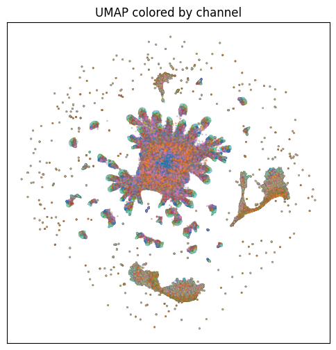
This view is one of the sanity checks I used for patch-level embeddings. Coloring by channel helped show whether local embeddings were mainly organizing around marker identity or something else.
The Patch-Level Problem
Patch embeddings were especially interesting, but they also created a practical problem. For each cell, the model produced many patch tokens per channel. With 11 channels, this quickly became huge.
A single 256 by 256 image with 16 by 16 patches gives 256 patches per channel. With 11 channels, that is 2816 patch embeddings per cell. Across thousands of cells, this becomes far too many points for a simple UMAP workflow.
So I had to reduce the problem. I tried balanced sampling across datasets and looked at smaller subsets of patches. I also looked at central patches separately, because those are more likely to contain useful cell signal than image corners or background-heavy regions.
Then another issue showed up: not every patch contained meaningful signal. Some regions were mostly background. To make the patch-level analysis cleaner, I computed patch intensities and used an Otsu-style threshold to filter low-signal patches.
Even after that, the patch embeddings were not only about biology.
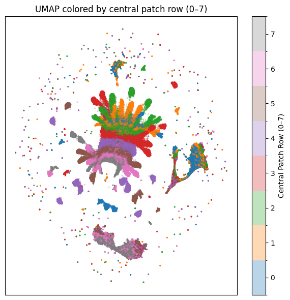
Coloring the same kind of embedding by patch row made it clear that spatial position mattered a lot. That was a good lesson. If an embedding separates nicely, the next question is always: separates by what?
In this case, some structure came from where the patch was located in the crop, not only from the biological marker or condition.
Cross-Dataset Checks
I also tried a small cross-dataset comparison using shared markers. The idea was to ask whether matching markers from different microscopy datasets would land in a shared embedding space.
The short answer was: not really, at least not cleanly in this setup.
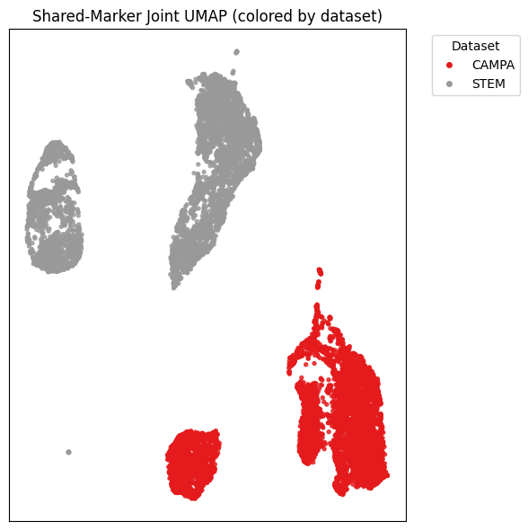
Even when looking at shared markers, the embeddings still separated strongly by dataset. That does not mean the model failed completely. But it does suggest that dataset origin, imaging setup, cell type, and preprocessing still have a big influence. A frozen pretrained model does not automatically remove those differences.
What Was Hard
The hardest part was not one big algorithmic problem. It was lots of small, practical decisions that each affected the result.
Choosing channels was one of them. The paper model was built to be flexible, but the actual inference path I used still came with constraints. Our data had richer channel panels than the model input I was working with, so I had to pick a subset and then be honest about what that means.
Another hard part was scale. Global embeddings were easy to manage. Patch embeddings were much heavier. They were useful because they gave a more local view, but they also forced me to think about sampling, filtering, and whether the plots were showing signal or just technical structure.
The interpretation was probably the most important part. It is tempting to look at a colorful UMAP and immediately tell a story. But the more I checked the embeddings from different angles, the more careful I had to be. Sometimes the structure was biological. Sometimes it was channel identity. Sometimes it was spatial position. Sometimes it was probably dataset-specific effects.
That was frustrating at times, but also the part I enjoyed most. It felt like slowly learning how to ask better questions of the model.
What I Took Away
My main takeaway is that pretrained microscopy foundation models are useful, but they still need careful handling.
CA-MAE gave us embeddings that were interesting enough to analyze. It could capture some broad structure, and the different representation levels made it possible to inspect the data from several angles. But in this project, the embeddings did not cleanly solve the harder parts for free. Subtle perturbation effects were difficult. Cross-dataset alignment was limited. Channel and spatial effects were strong.
I also learned that a lot of the work sits between the paper and the plot. The paper gives you the model idea. The real project asks: What does my input tensor look like? Which channels should I use? How do I avoid fooling myself with background patches? What exactly is this cluster separating?
That made the project fun. It was not just running a model and collecting a result. It was a lot of small decisions, sanity checks, and back-and-forth between code, images, and biology. I came away with more respect for how hard it is to make representation learning useful on real scientific data.